TL;DR
- Muon is the de facto matrix aware optimizer for LLM pretraining, which is basically next token classification on text via supervised learning. Muon orthogonalizes the momentum matrix through a few Newton Schulz (NS) iterations, pushing every singular value of the momentum to one.
- When we move beyond LLM pretraining along three axes (a different modality, a different loss, or a different learning paradigm), Muon’s uniform spectral whitening turns out to be the wrong inductive bias.
- We propose Pion (sPectral hIgh pass Optimization on momeNtum), a drop in replacement for Muon’s NS iteration. It changes only the polynomial coefficients used inside NS, keeps the same per step cost, and realizes a sharp spectral high pass that anchors the informative leading singular values at one while suppressing the noisy tail toward zero.
Try It: Where Does a Singular Value Go?
Background
Muon
Muon is a matrix aware optimizer that has gained wide adoption in LLM pretraining. Its entire construction is built around a single observation: treating the momentum as a matrix rather than a flat vector, the natural notion of steepest descent under the spectral norm orthogonalizes the momentum’s singular vectors and pushes every nonzero singular value to one.
For a weight matrix \(\boldsymbol{\Theta} \in \mathbb{R}^{m \times n}\), given a stochastic gradient \(\mathbf{G}_t\) and a momentum buffer \(\mathbf{M}_t = \mu \mathbf{M}_{t-1} + \mathbf{G}_t\), Muon performs the steepest descent step under the spectral norm:
\[\boldsymbol{\Theta}_t = \boldsymbol{\Theta}_{t-1} - \eta \, \mathrm{msign}(\mathbf{M}_t).\]If \(\mathbf{M} = \mathbf{U} \boldsymbol{\Sigma} \mathbf{V}^\top\) is the compact SVD, then
\[\mathrm{msign}(\mathbf{M}) = \mathbf{U}\, \mathrm{sign}(\boldsymbol{\Sigma})\, \mathbf{V}^\top = \mathbf{U} \mathbf{V}^\top.\]Every nonzero singular value is mapped to one. This is uniform spectral whitening. Computing an SVD per step is too expensive at scale, so Muon approximates \(\mathrm{msign}\) by a small number of Newton Schulz (NS) iterations. After normalizing the input as \(\mathbf{X} \leftarrow \mathbf{X} / (\|\mathbf{X}\|_F + \epsilon)\), each NS step applies an odd quintic matrix polynomial,
\[\mathbf{X} \leftarrow a\, \mathbf{X} + b\, \mathbf{X}\mathbf{X}^\top \mathbf{X} + c\, \mathbf{X}(\mathbf{X}^\top \mathbf{X})^2,\]with the canonical coefficients \((a, b, c) = (3.4445,\ -4.7750,\ 2.0315)\). By the identity \(\mathbf{X}(\mathbf{X}^\top \mathbf{X})^j = \mathbf{U}\, \boldsymbol{\Sigma}^{2j+1}\, \mathbf{V}^\top\), an NS step preserves the singular vectors and reshapes each singular value through a scalar polynomial on \([0, 1]\):
\[f(\sigma;\, a, b, c) \,\triangleq\, a\sigma + b\sigma^3 + c\sigma^5.\]So designing an NS iteration reduces to designing \(f\) on \([0, 1]\). Muon’s NS is constructed so that repeated application drives every \(\sigma \in (0, 1]\) toward one. The shape of this scalar map (and Pion’s eventual replacement for it) is the central object we visualize later in Figure 1.
Three Axes Beyond Pretraining
LLM pretraining is typically optimized with a next token prediction loss; more concretely, the task is classification, the modality is text only, and the paradigm is supervised learning. When per token supervision is dense and accurate, pushing every singular value to one is a reasonable default. But LLM pretraining is only one part of deep learning, and how Muon behaves along different modalities, losses, and learning paradigms remains an open question worth exploring.
Motivation
We consider two settings: VLA and RLVR. VLA simultaneously changes the modality and the loss (introducing the vision and action modalities and replacing classification with regression loss); RLVR changes only the learning paradigm (replacing supervised learning with reinforcement learning). Through gradient rank and signal-to-noise ratio analyses, we find that Muon transfers poorly to both the action modality and reinforcement learning.
Beyond Modality and Loss: VLA
A VLA model is factorized into a vision encoder, a language backbone, and an action head. The vision and language modules take text instructions and images as input, while the action head is a new modality whose output is the robot’s actions. Correspondingly, the action head is trained with a non-classification loss: either \(\ell_1\) regression (e.g., VLA Adapter) or flow matching (e.g., VLANeXt). The “action modality” and “regression-style loss” choices are tightly coupled by construction.
We measure the spectral structure of each module’s gradient via the effective rank (erank) of \(\mathbf{G} \in \mathbb{R}^{m \times n}\):
\[\mathrm{erank}(\mathbf{G}) \,\triangleq\, \exp\!\Big( H(\mathbf{p}) \Big), \quad H(\mathbf{p}) = -\sum_{i=1}^n p_i \log p_i, \quad p_i = \frac{\sigma_i(\mathbf{G})}{\sum_j \sigma_j(\mathbf{G})}.\]A higher erank means gradient energy is spread across many singular directions; a lower erank means it concentrates in a few dominant ones.
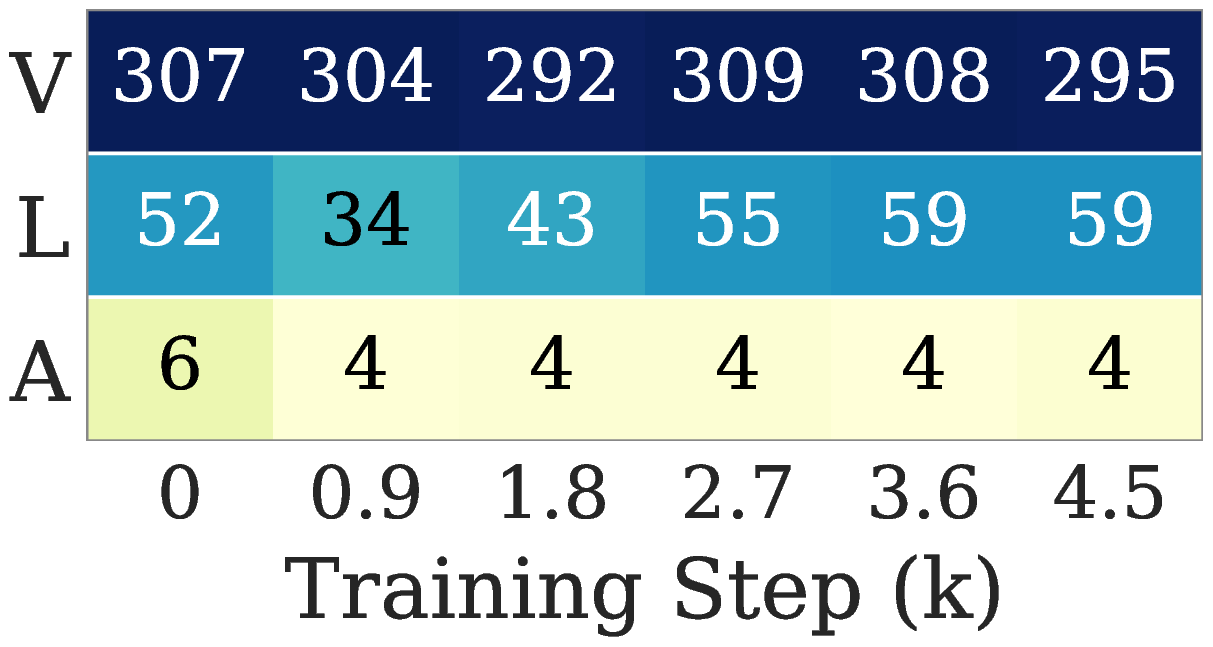
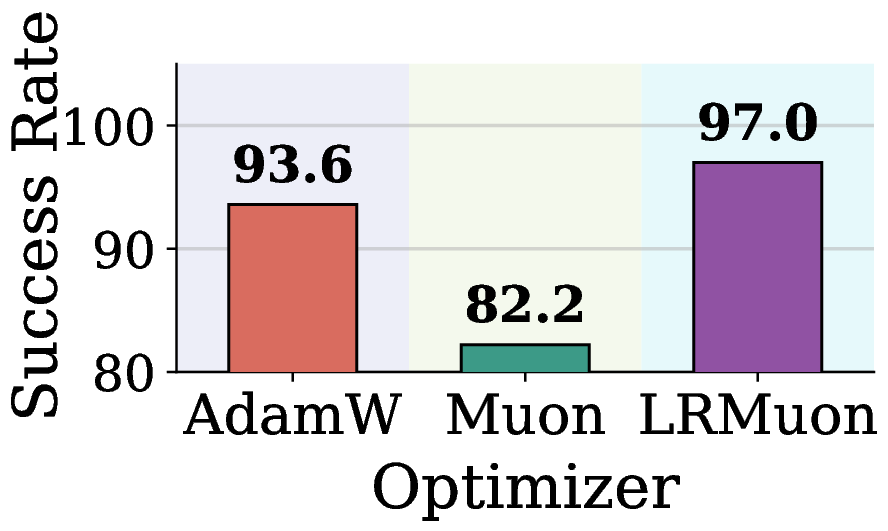
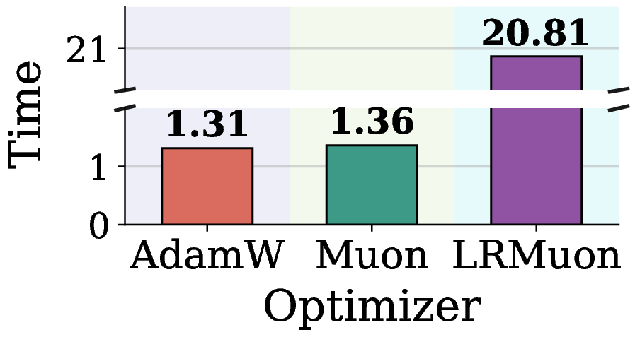
Figure 2. Limitations of Muon in VLA training (VLA Adapter on LIBERO Object). (a) Per module gradient erank along the training trajectory. (b)(c) Test success rate and total training time at 4.5k steps, with vision and language fixed at AdamW; only the action module optimizer differs.
The ordering in Figure 2(a) is stable across training: vision is the highest, language sits in the middle, and the action gradient is consistently the lowest. The intuition is twofold: vision and text inputs carry far richer information per sample, whereas an action vector only needs 7 degrees of freedom to express; on top of that, the action head is trained with a regression loss, whose output space is much smaller than the discrete-token space of language and vision, so its gradient is strongly low-rank in nature. When Muon is applied uniformly to such a low-erank gradient, it lifts the weak noise tail to the same magnitude as the few informative leading directions, and the resulting update is dominated by spectral floor noise. Consequently, Figure 2(b) shows Muon underperforming AdamW on the action head. A natural workaround, Low-Rank Muon (LRMuon), projects the momentum onto a top \(k\) subspace via SVD or Gaussian sketching before NS. LRMuon recovers the success rate, but Figure 2(c) shows that the explicit projection inflates wall clock by about an order of magnitude, and forces a fixed rank \(k\) that cannot adapt across layers and steps.
Limitation 1 (modality + loss). Conventional Muon does not adapt to the rank heterogeneity introduced by new modalities and non-classification losses. Explicit low-rank projection recovers the success rate but at the cost of scalability.
Beyond Learning Paradigm: RLVR
RLVR keeps the LLM and the text modality; only the learning paradigm changes: a token-level supervised loss (as in SFT) is replaced by a trajectory-level policy gradient against a verifiable reward (as in GRPO). To compare the two paradigms on the same footing, we measure the per-step gradient signal-to-noise ratio on a given layer’s weight matrix:
\[\mathrm{SNR}(\mathbf{G}) \,\triangleq\, \frac{\|\mathbb{E}[\mathbf{G}]\|_F^2}{\mathbb{E}\big[\,\|\mathbf{G} - \mathbb{E}[\mathbf{G}]\|_F^2\,\big]}.\]Two structural reasons explain the SNR gap in Figure 3(a). First, coarser supervision granularity: SFT uses token-level teacher signals, while GRPO uses trajectory-level rewards, so each token receives a much sparser learning signal. Second, stabilization mechanisms: importance sampling, clipping, and group-relative normalization reweight or zero out parts of the per-token gradients, further inflating variance. When Muon is applied on top of these low-SNR gradients, the uniform whitening lifts the noisy directions to the same magnitude as the informative ones, and the policy collapses within a few steps, as shown in Figure 3(b).
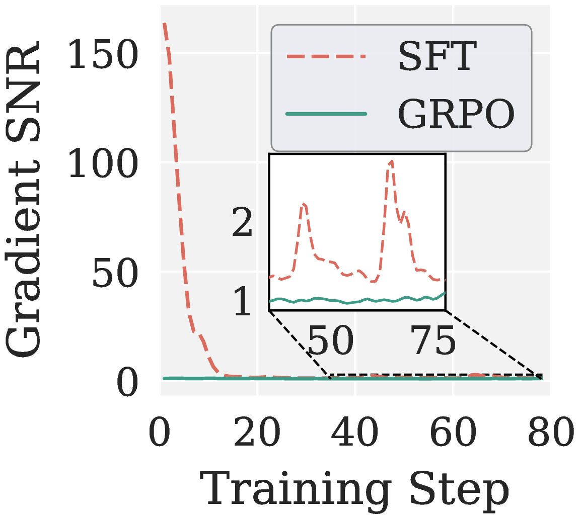
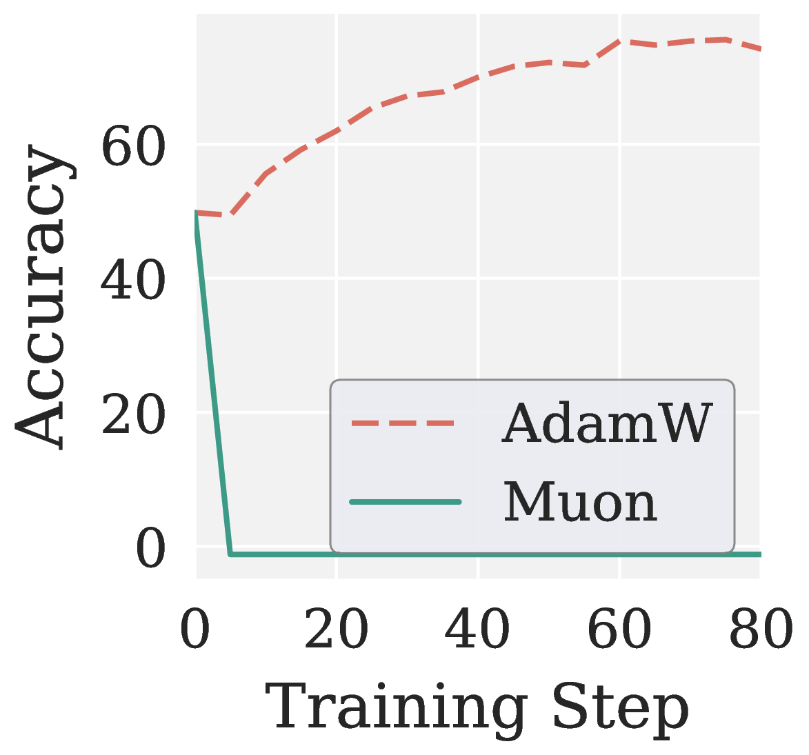
Figure 3. RLVR diagnosis on Qwen3 1.7B (MATH levels 3 to 5). (a) GRPO has substantially lower gradient SNR than SFT throughout training. (b) Under GRPO, AdamW improves steadily while Muon collapses to near zero accuracy within a few steps.
Limitation 2 (learning paradigm). Muon’s uniform spectral whitening amplifies noisy directions in low-SNR RLVR gradients, making it unsuitable for noise-sensitive post-training.
Method
Limitations 1 and 2 come from different sources (low effective rank along the modality / loss axes, low SNR along the learning paradigm axis), yet they share one spectral signature. In the SVD of \(\mathbf{M}_t\), the few leading singular values carry the informative descent direction, while the long tail of small singular values is dominated by noise: a spectral floor when erank is low, stochastic estimation noise when SNR is low. Muon’s \(\mathrm{msign}\) lifts the tail to the magnitude of the head and corrupts the update in both regimes. The natural remedy is a spectral high pass: anchor the informative head near one and contract the noisy tail toward zero.
High-Pass NS
Since each NS step reshapes \(\sigma \in [0, 1]\) through the scalar polynomial \(f(\sigma; a, b, c) = a\sigma + b\sigma^3 + c\sigma^5\), designing an NS iteration reduces to designing \(f\). A single such polynomial cannot produce a sharp high pass on the unit interval, so Pion splits the default \(k = 5\) NS steps into two stages with different coefficients:
- a Promotion polynomial \(f_{\mathrm{p}}\) applied for \(k_{\mathrm{p}}\) steps, which lifts dominant singular values toward one while preserving their relative order;
- a Suppression polynomial \(f_{\mathrm{s}}\) applied for \(k_{\mathrm{s}} = k - k_{\mathrm{p}}\) steps, which pins large singular values near one and contracts smaller ones toward zero.
The cutoff is controlled by the single hyperparameter \(k_{\mathrm{p}} \in \{0, 1, \ldots, 5\}\).
We require three constraints on \(f_{\mathrm{p}}\): (P1) fixed point \(f_{\mathrm{p}}(1) = 1\); (P2) first order stationarity \(f_{\mathrm{p}}'(1) = 0\); and (P3) boundary concavity \(f_{\mathrm{p}}''(1) \leq 0\), which together with (P2) ensures \(\sigma = 1\) is a maximum so that the iteration does not curve upward past one near the boundary. Solving (P1) and (P2) leaves a one parameter family. Combining (P3) with monotonicity on \([0, 1]\) carves out the feasible interval \(a_{\mathrm{p}} \in [0, 1.875]\). Since \(f_{\mathrm{p}}'(0) = a_{\mathrm{p}}\) controls how strongly each step lifts small singular values, we pick the largest feasible slope, which uniquely determines the polynomial:
\[f_{\mathrm{p}}(\sigma) = 1.875\, \sigma \,-\, 1.25\, \sigma^3 \,+\, 0.375\, \sigma^5.\]A pleasant byproduct is that the derivative becomes a perfect square, \(f_{\mathrm{p}}'(\sigma) = 1.875\, (1 - \sigma^2)^2 \geq 0\), so monotonicity on \([0, 1]\) holds automatically.
The Suppression polynomial inherits \(f_{\mathrm{s}}(1) = 1\) and \(f_{\mathrm{s}}'(1) = 0\), and adds a spectral filtering condition \(f_{\mathrm{s}}'(0) = 0\). Removing the linear term near the origin forces small singular values to be driven to zero by the higher order terms. The unique solution is
\[f_{\mathrm{s}}(\sigma) = 2.5\, \sigma^3 \,-\, 1.5\, \sigma^5.\]Chaining \(k_{\mathrm{p}}\) Promotion steps with \(k_{\mathrm{s}}\) Suppression steps gives Pion’s high-pass NS iteration. Fixing \(k = 5\) preserves Muon’s per-step cost. Figure 1 compares Muon NS, Promotion, Suppression, and the resulting Pion high-pass NS profile: a sharp transition between a pinned region near one and a filtered region near zero, with \(k_{\mathrm{p}}\) controlling the cutoff. Empirically, suppression-dominant allocations with \(k_{\mathrm{s}} \geq 3\) work best for both VLA and RLVR.
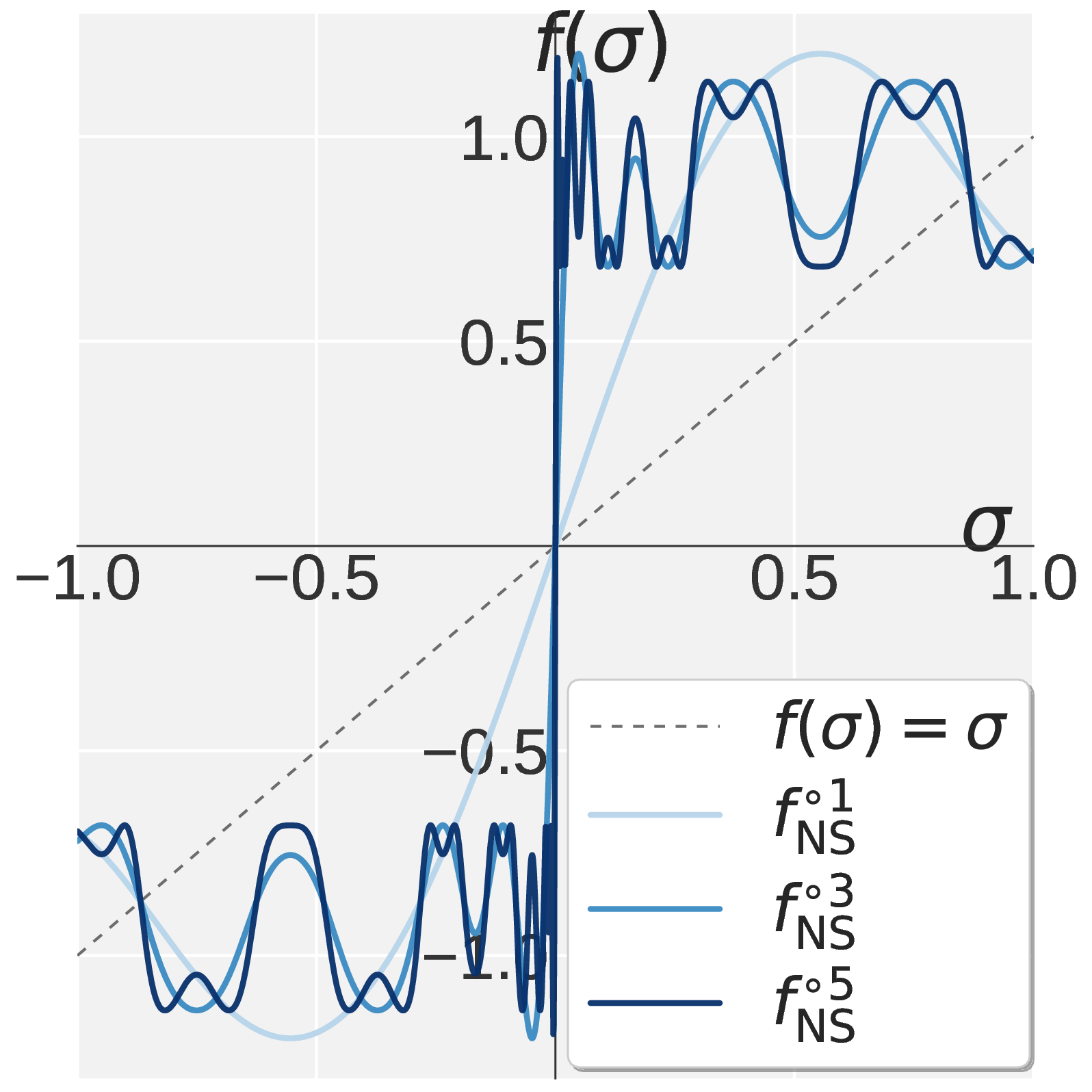
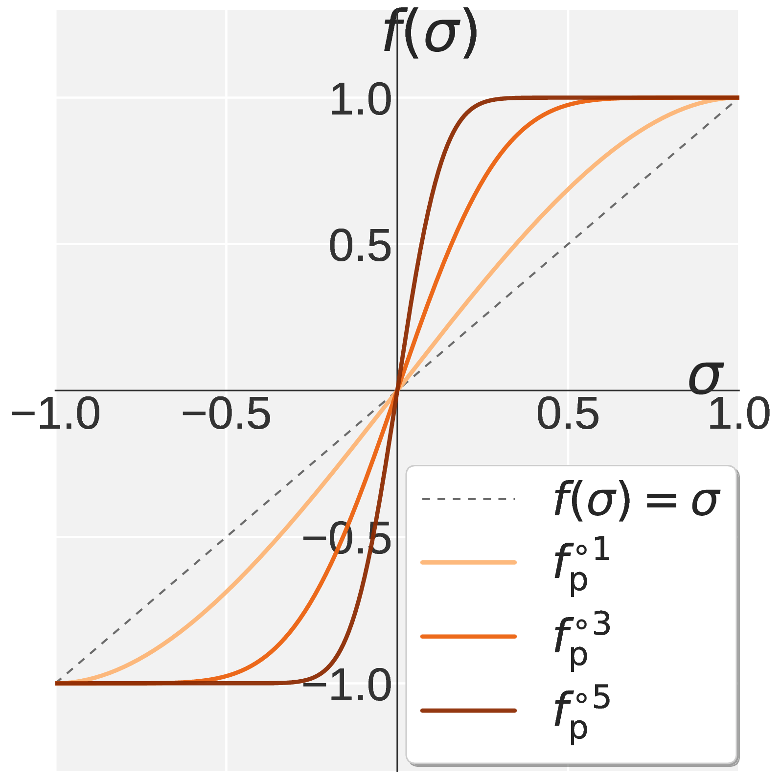
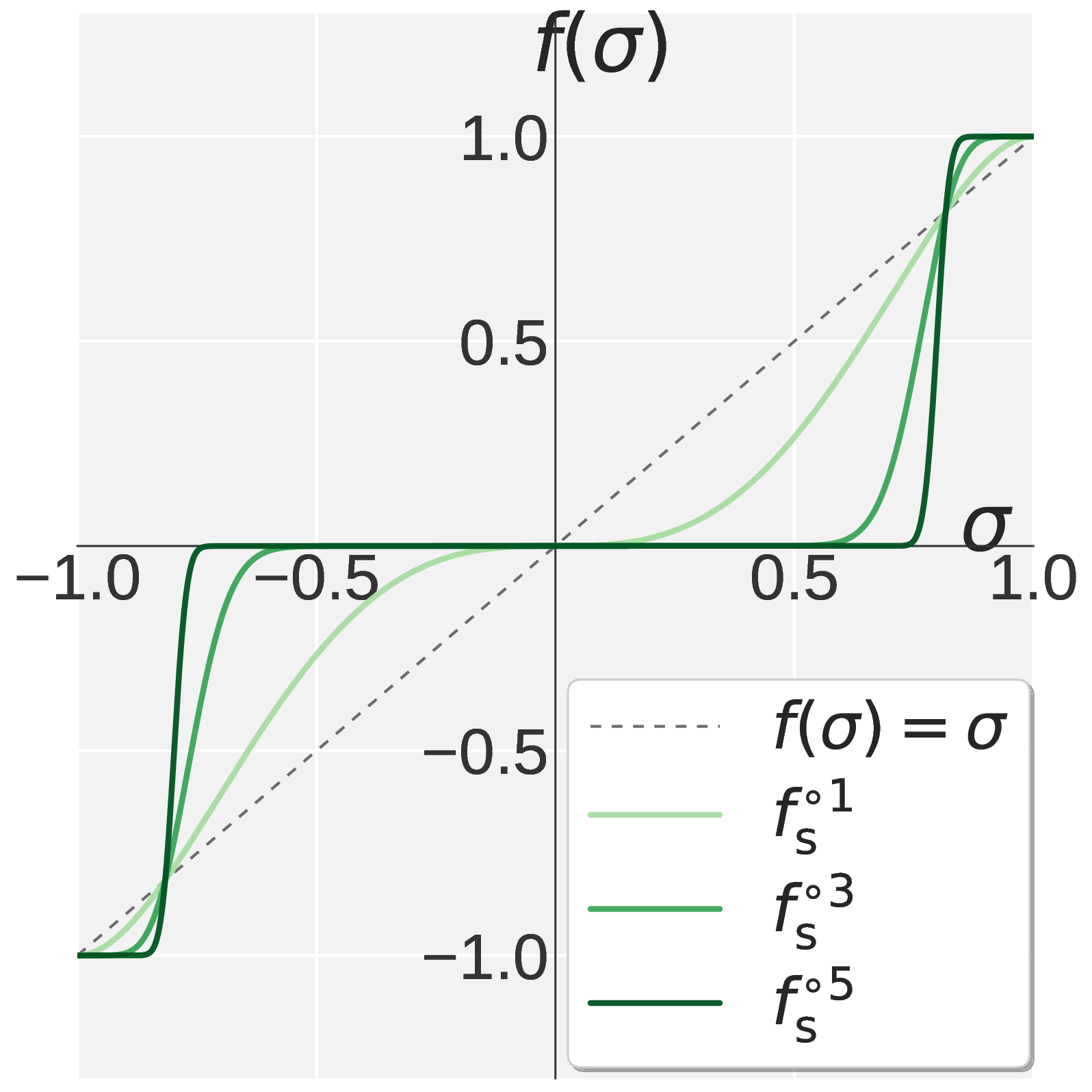
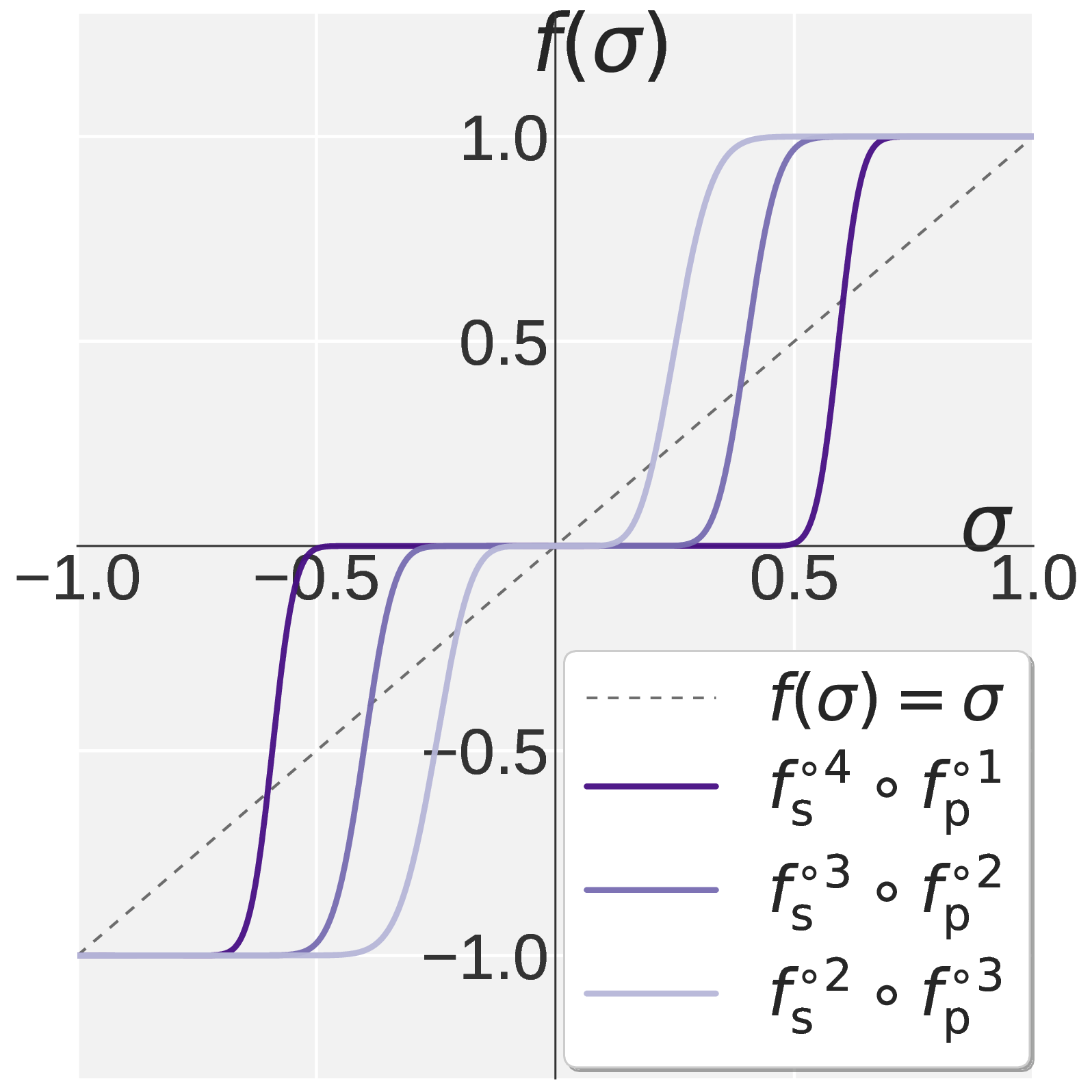
Figure 1. Visualization of \(f(\sigma)\) on \(\sigma \in [0, 1]\). Muon (a) drives every singular value toward one. Pion combines Promotion (b) with Suppression (c) to obtain the high pass profile in (d).
Per-Head Mode for RLVR
So far the high-pass NS has been applied to each per-layer momentum \(\mathbf{M}_t \in \mathbb{R}^{m \times n}\) as a single block, exactly mirroring Muon; we call this the default mode. We find that this does not transfer well to RLVR. RLVR starts from a model that has already been pretrained (or SFT’d), whose attention layers exhibit substantial per-head heterogeneity in \(\|\mathbf{W}_Q^h\|_F\), \(\|\mathbf{W}_K^h\|_F\), \(\|\mathbf{W}_V^h\|_F\), and \(\|\mathbf{W}_O^h\|_F\). This heterogeneity jointly governs the forward outputs and the backward gradients, so different heads should naturally receive updates at different scales.
To respect this structure, Pion adds a per-head mode that first reshapes each attention projection along the head dimension into per-head sub-matrices and then runs the two-stage high-pass NS independently on each. Formally, with \(H\) attention heads and per-head dimension \(d_k\), each attention projection (Q / K / V / O) admits a canonical reshape along the head axis,
\[\mathbf{M}_t \;\xrightarrow{\;\mathrm{Reshape}\;}\; \{\mathbf{M}_t^h\}_{h=1}^{H}, \qquad \mathbf{M}_t^h \in \mathbb{R}^{d \times d_k}.\]The per-head mode then applies the full two-stage high-pass NS independently on each \(\mathbf{M}_t^h\): a per-head Frobenius pre-normalization \(\mathbf{X}^h \leftarrow \mathbf{M}_t^h / (\|\mathbf{M}_t^h\|_F + \epsilon)\), followed by \(k_{\mathrm{p}}\) Promotion steps and \(k_{\mathrm{s}}\) Suppression steps, and finally a reshape of \(\{\mathbf{X}^h\}_{h=1}^H\) back to a single \(\mathbf{X} \in \mathbb{R}^{m \times n}\). Because \(\mathbf{X}^h (\mathbf{X}^h)^\top \mathbf{X}^h\) is naturally batched over \(h\) on GPU, the only extra cost over the default mode is the reshape itself.
Figure 4(a) makes the default-mode failure concrete on Qwen3 1.7B: the pre-RLVR cross-head variance \(\mathrm{Var}_h(\|\mathbf{W}_{0,Q}^h\|_F)\) is non-negligible across all 28 layers (top), yet under default-mode Pion the update variance \(\mathrm{Var}_h(\|\mathbf{W}_{*,Q}^h - \mathbf{W}_{0,Q}^h\|_F)\) collapses to near zero (bottom). In other words, a single Frobenius pre-normalization plus a single NS chain over the whole projection equalizes the update scale across heads and mixes head-specific directions, so every head ends up with an almost identical update and the inter-head heterogeneity is erased. By contrast, the per-head mode restores a layer-dependent, head-specific update profile.
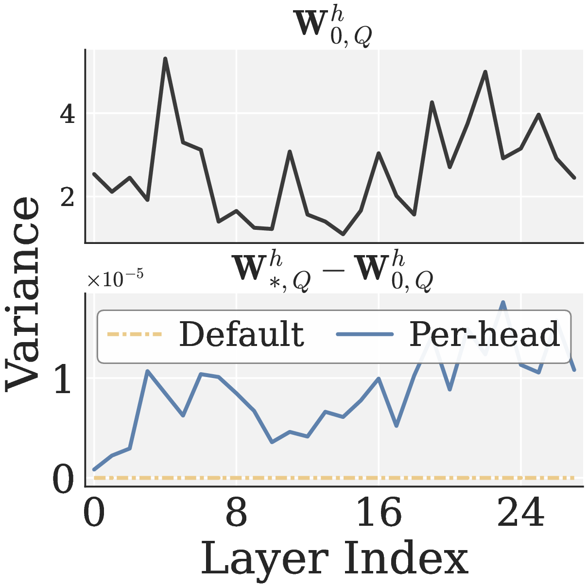
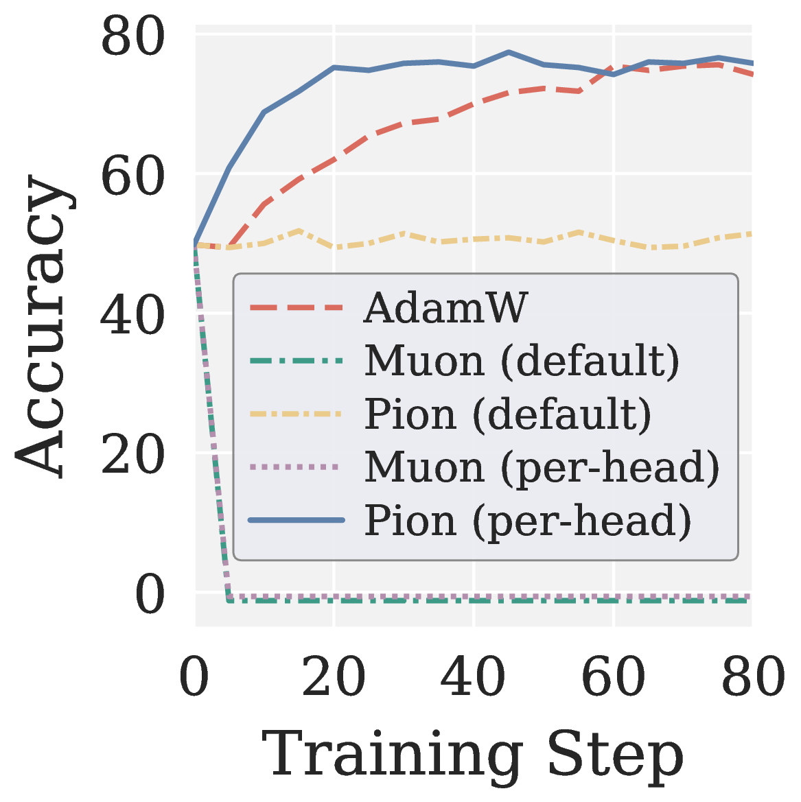
Figure 4. Effect of per-head high-pass NS on RLVR (Qwen3 1.7B, GRPO on MATH levels 3 to 5). (a) Cross-head Q projection variance: pre-RLVR weight \(\mathrm{Var}_h(\|\mathbf{W}_{0,Q}^h\|_F)\) (top) and post-RLVR update \(\mathrm{Var}_h(\|\mathbf{W}_{*,Q}^h - \mathbf{W}_{0,Q}^h\|_F)\) for default vs. per-head Pion (bottom). (b) MATH500 accuracy of AdamW, Muon (default vs. per-head), and Pion (default vs. per-head).
At this point, Pion’s per-head high-pass NS bundles two design choices: the spectral high pass and the per-head reshape. A natural follow-up question is which of the two is doing the heavy lifting. We find that the two are complementary but not symmetric. The spectral high pass is the primary driver: in Figure 4(b), even if we apply the same reshape on top of Muon’s NS, the resulting per-head Muon still collapses, because injecting the noise tail head-by-head is just as harmful as injecting it on the whole matrix. The per-head reshape is the auxiliary mechanism, used to preserve the per-head heterogeneity inherited from the pretrained (or SFT’d) attention layers. We do not use per-head mode for VLA: there the action head is trained from scratch, with no pretrained multi-head attention structure to preserve.
Algorithms
For reference, we write out the full procedures below. Algorithm 1 is Muon’s standard NS iteration. Pion only replaces the inner NS loop with a two stage high pass version: Algorithm 2 is the default mode used for VLA training; Algorithm 3 is the per head mode used for RLVR post training. The total iteration count is fixed to (k = 5), split into (k_{\mathrm{p}}) Promotion steps and (k_{\mathrm{s}} = k - k_{\mathrm{p}}) Suppression steps. Pion vs. Muon per head specific
- \(\mathbf{M}_0 \leftarrow \mathbf{0}\)
- for \(t = 1, 2, \dots\) do
- \(\mathbf{G}_t \leftarrow \nabla_{\boldsymbol{\Theta}} \mathcal{L}_t(\boldsymbol{\Theta}_{t-1})\)
- \(\mathbf{M}_t \leftarrow \mu\, \mathbf{M}_{t-1} + \mathbf{G}_t\)
- \(\mathbf{X} \leftarrow \mathbf{M}_t / (\lVert \mathbf{M}_t \rVert_F + \epsilon)\)spectral pre-norm
- for \(i = 1, \dots, k\) do\((a, b, c) = (3.4445, -4.7750, 2.0315)\)
- \(\mathbf{X} \leftarrow a\mathbf{X} + b\mathbf{X}\mathbf{X}^\top\mathbf{X} + c\mathbf{X}(\mathbf{X}^\top\mathbf{X})^2\)
- end for
- \(\boldsymbol{\Theta}_t \leftarrow \boldsymbol{\Theta}_{t-1} - \eta\, \mathbf{X}\)
- end for
- return \(\boldsymbol{\Theta}_t\)
- \(k_{\mathrm{s}} \leftarrow 5 - k_{\mathrm{p}}\)split \(k = 5\) into \(k_{\mathrm{p}} + k_{\mathrm{s}}\)
- \(\mathbf{M}_0 \leftarrow \mathbf{0}\)
- for \(t = 1, 2, \dots\) do
- \(\mathbf{G}_t \leftarrow \nabla_{\boldsymbol{\Theta}} \mathcal{L}_t(\boldsymbol{\Theta}_{t-1})\)
- \(\mathbf{M}_t \leftarrow \mu\, \mathbf{M}_{t-1} + \mathbf{G}_t\)
- \(\mathbf{X} \leftarrow \mathbf{M}_t / (\lVert \mathbf{M}_t \rVert_F + \epsilon)\)spectral pre-norm
- for \(i = 1, \dots, k_{\mathrm{p}}\) dostage 1: Promotion, \((a_{\mathrm{p}}, b_{\mathrm{p}}, c_{\mathrm{p}}) = (1.875, -1.25, 0.375)\)
- \(\mathbf{X} \leftarrow a_{\mathrm{p}}\mathbf{X} + b_{\mathrm{p}}\mathbf{X}\mathbf{X}^\top\mathbf{X} + c_{\mathrm{p}}\mathbf{X}(\mathbf{X}^\top\mathbf{X})^2\)
- end for
- for \(j = 1, \dots, k_{\mathrm{s}}\) dostage 2: Suppression, \((a_{\mathrm{s}}, b_{\mathrm{s}}, c_{\mathrm{s}}) = (0, 2.5, -1.5)\)
- \(\mathbf{X} \leftarrow a_{\mathrm{s}}\mathbf{X} + b_{\mathrm{s}}\mathbf{X}\mathbf{X}^\top\mathbf{X} + c_{\mathrm{s}}\mathbf{X}(\mathbf{X}^\top\mathbf{X})^2\)
- end for
- \(\boldsymbol{\Theta}_t \leftarrow \boldsymbol{\Theta}_{t-1} - \eta\, \mathbf{X}\)
- end for
- return \(\boldsymbol{\Theta}_t\)
- \(k_{\mathrm{s}} \leftarrow 5 - k_{\mathrm{p}}\)split \(k = 5\) into \(k_{\mathrm{p}} + k_{\mathrm{s}}\)
- \(\mathbf{M}_0 \leftarrow \mathbf{0}\)
- for \(t = 1, 2, \dots\) do
- \(\mathbf{G}_t \leftarrow \nabla_{\boldsymbol{\Theta}} \mathcal{L}_t(\boldsymbol{\Theta}_{t-1})\)
- \(\mathbf{M}_t \leftarrow \mu\, \mathbf{M}_{t-1} + \mathbf{G}_t\)
- \(\{\mathbf{M}_t^h\}_{h=1}^{H} \leftarrow \mathrm{Reshape}(\mathbf{M}_t)\)split attention along head dim
- \(\mathbf{X}^h \leftarrow \mathbf{M}_t^h / (\lVert \mathbf{M}_t^h \rVert_F + \epsilon),\ \forall\, h\)per head pre-norm
- for \(i = 1, \dots, k_{\mathrm{p}}\) dostage 1: Promotion, batched over \(H\)
- \(\mathbf{X}^h \leftarrow a_{\mathrm{p}}\mathbf{X}^h + b_{\mathrm{p}}\mathbf{X}^h(\mathbf{X}^h)^\top\mathbf{X}^h + c_{\mathrm{p}}\mathbf{X}^h\bigl((\mathbf{X}^h)^\top\mathbf{X}^h\bigr)^2\)
- end for
- for \(j = 1, \dots, k_{\mathrm{s}}\) dostage 2: Suppression, batched over \(H\)
- \(\mathbf{X}^h \leftarrow a_{\mathrm{s}}\mathbf{X}^h + b_{\mathrm{s}}\mathbf{X}^h(\mathbf{X}^h)^\top\mathbf{X}^h + c_{\mathrm{s}}\mathbf{X}^h\bigl((\mathbf{X}^h)^\top\mathbf{X}^h\bigr)^2\)
- end for
- \(\mathbf{X} \leftarrow \mathrm{Reshape}^{-1}(\{\mathbf{X}^h\}_{h=1}^{H})\)rejoin per head matrices
- \(\boldsymbol{\Theta}_t \leftarrow \boldsymbol{\Theta}_{t-1} - \eta\, \mathbf{X}\)
- end for
- return \(\boldsymbol{\Theta}_t\)
Takeaway. Pion is a drop in replacement for Muon’s NS iteration. Same control flow, same per step cost; only the polynomial coefficients change.
Experiments
We evaluate Pion in two settings:
- VLA training: two architectures, \(\ell_1\)-regression based VLA Adapter and flow-matching based VLANeXt, with LIBERO and LIBERO Plus as benchmarks.
- RLVR post-training: GRPO and GMPO on Qwen3 1.7B and Qwen3 4B, with MATH and GSM8K as benchmarks.
VLA
VLA Adapter on LIBERO. We first compare AdamW, Muon, and Pion on VLA Adapter across the four LIBERO task suites (Object, Spatial, Goal, Long) under a fixed per-suite training budget (1,500 steps for Object, 15,000 steps for the others), together with a finer learning curve on Object.

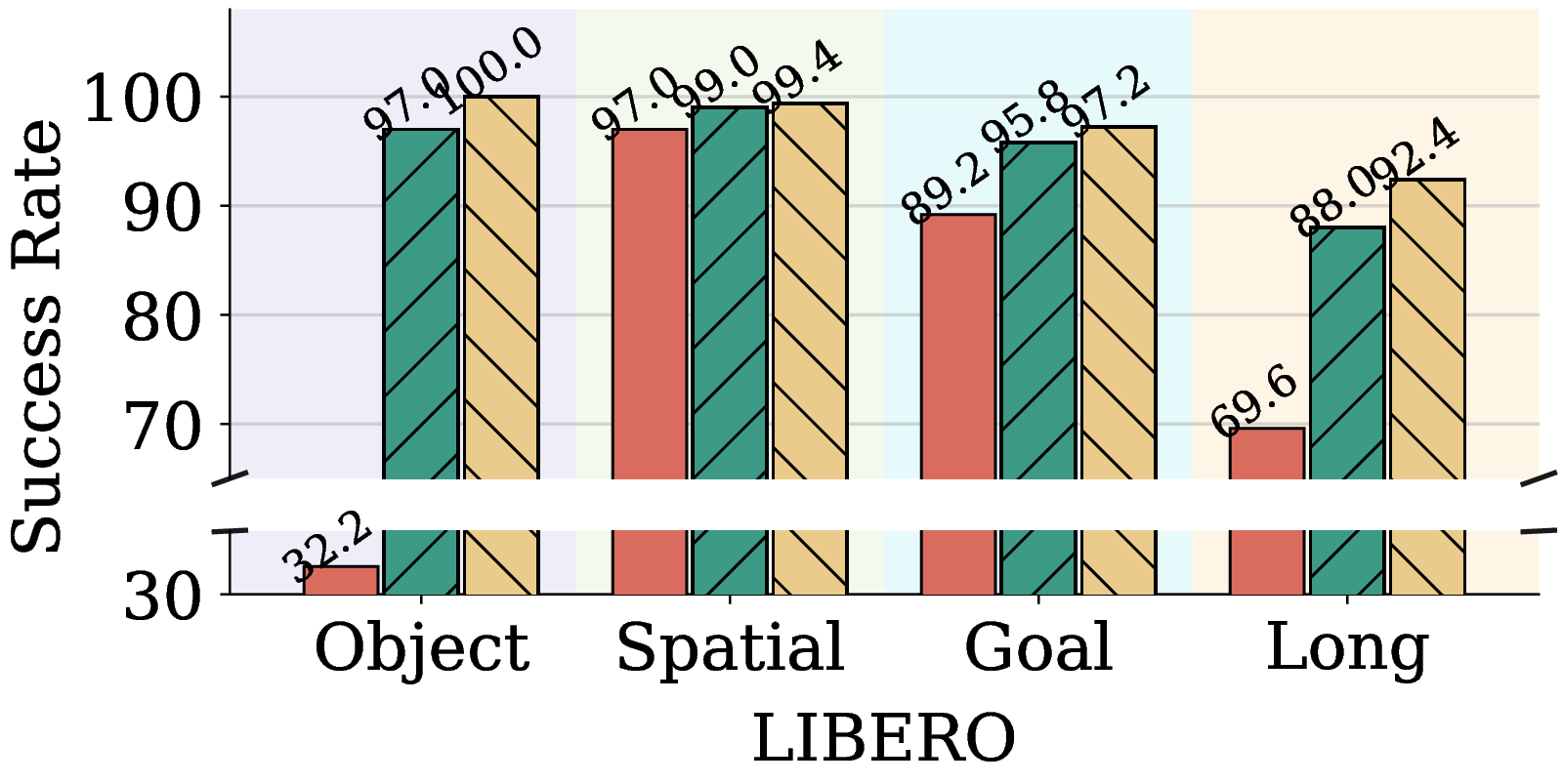
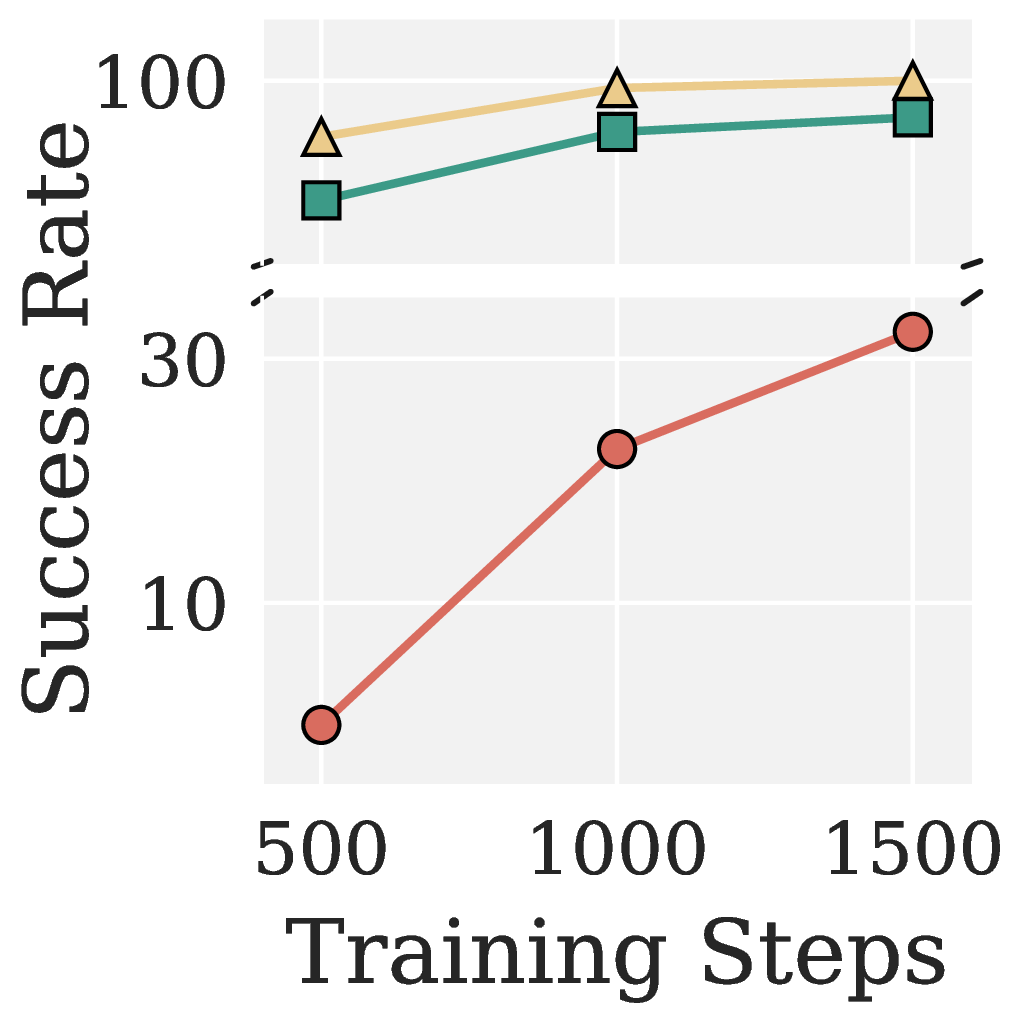
Figure 5. AdamW, Muon, and Pion for VLA Adapter on LIBERO. (a) Test success rates on LIBERO Object, Spatial, Goal, and Long at a fixed training budget per suite (1,500 steps for Object, 15,000 steps for the others). (b) Test success rate vs. training steps on LIBERO Object.
Figure 5(a) shows that Pion comprehensively outperforms both Muon and AdamW on every suite. Figure 5(b) further zooms into the LIBERO Object learning curve: Pion reaches 95.4% success at 500 steps and saturates at 100% by 1,500 steps, while AdamW requires substantially more steps to catch up. This indicates that the spectral high pass substantially reduces the training cost needed to reach the high-success regime.
VLANeXt on LIBERO and LIBERO Plus. With flow matching, Pion not only achieves the best success rate on LIBERO but also retains its advantage on the more challenging LIBERO Plus split, particularly under the language (\(+9\) pts), noise (\(+6\) pts), and robot (\(+6\) pts) perturbations; see Table 1. This confirms our earlier picture that uniform whitening over-amplifies noise directions that do not generalize.
| Optimizer | LIBERO | LIBERO Plus | Background | Camera | Language | Layout | Light | Noise | Robot |
|---|---|---|---|---|---|---|---|---|---|
| AdamW | 79.45 | 64.57 | 68.97 | 70.38 | 54.50 | 61.80 | 76.35 | 66.37 | 47.04 |
| Muon | 93.65 | 72.34 | 82.72 | 68.00 | 77.53 | 76.21 | 86.17 | 69.98 | 57.36 |
| Pion (Ours) | 96.35 | 75.93 | 84.53 | 70.88 | 86.93 | 76.71 | 90.67 | 76.09 | 63.18 |
Table 1. AdamW, Muon, and Pion for VLANeXt on LIBERO and LIBERO Plus. Best in bold.
To make the LIBERO Plus gap concrete, we roll out the same LIBERO Plus episode under VLANeXt policies trained with each optimizer. AdamW and Muon fail at the grasp or placement stage, while Pion completes the task cleanly.
Video 1. Rollouts on the same LIBERO Plus episode (ep1373) under VLANeXt policies trained with the three optimizers. Only Pion reliably completes the task; AdamW and Muon fail in the grasp or placement stage.
RLVR
Across all eight RLVR settings (GRPO/GMPO × Qwen3 1.7B/4B × MATH/GSM8K; see Figure 6), Muon collapses to near-zero accuracy without exception. Pion not only recovers a meaningful training signal but also converges faster than AdamW.
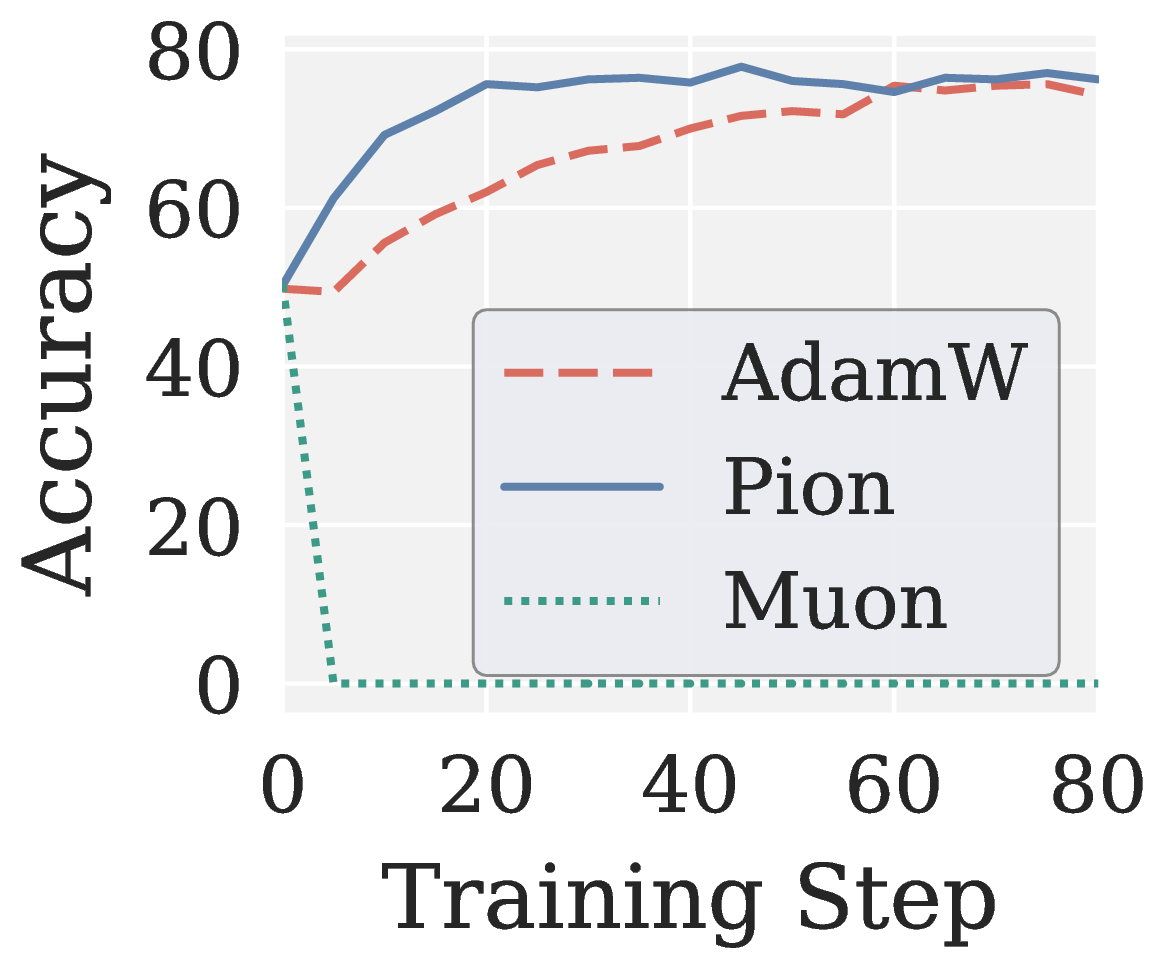
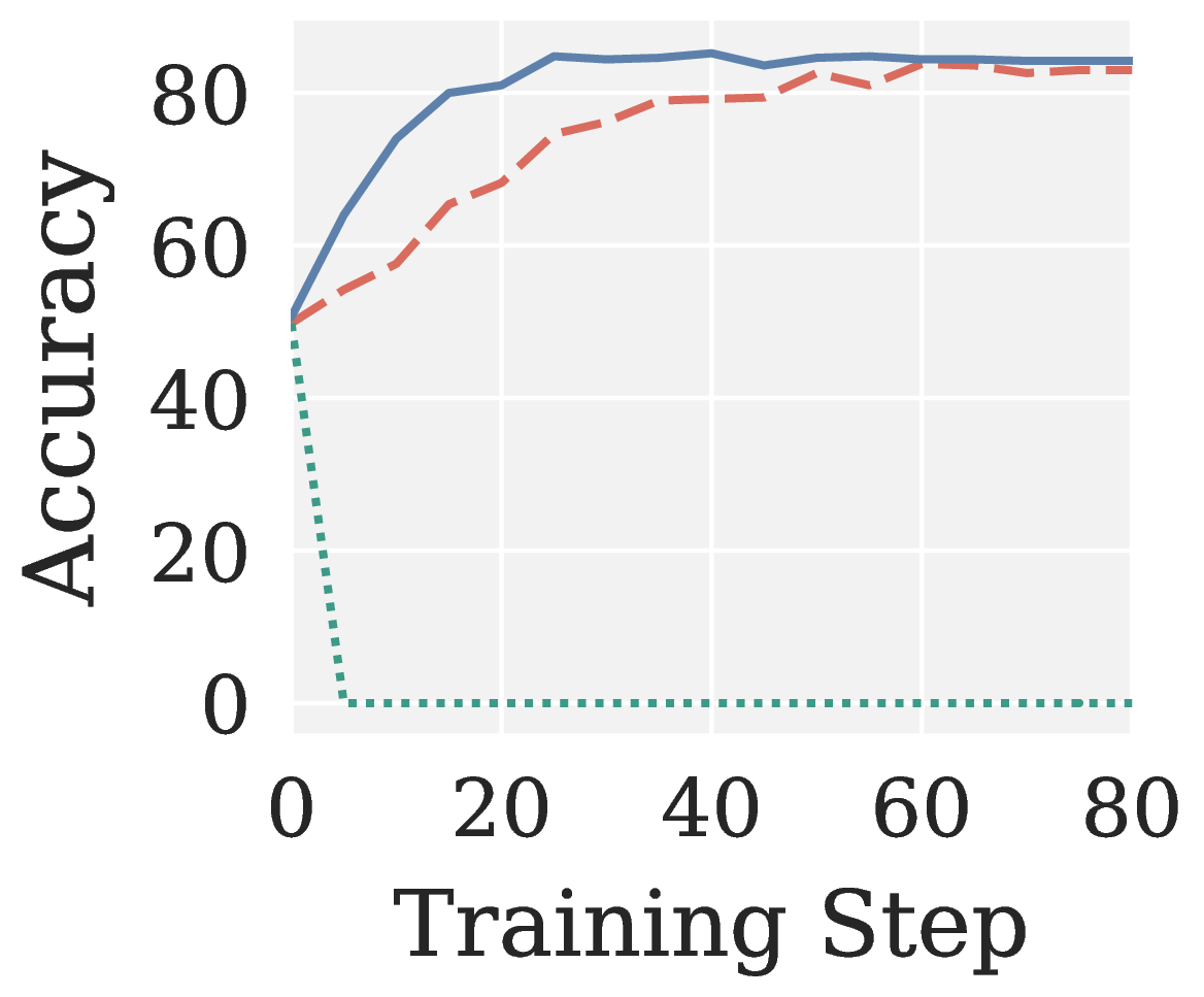
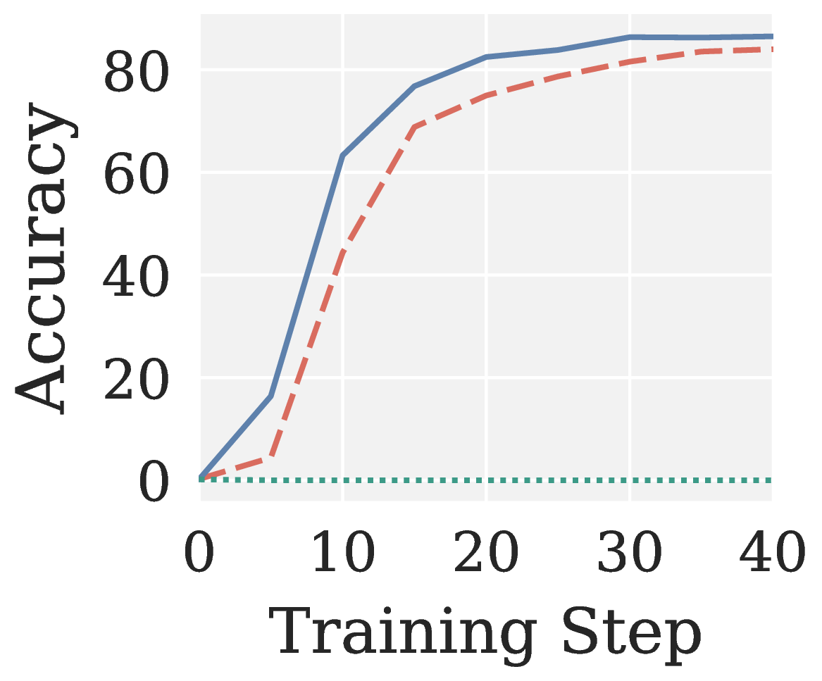
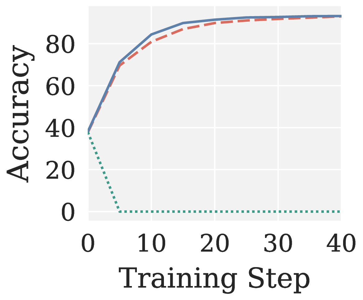
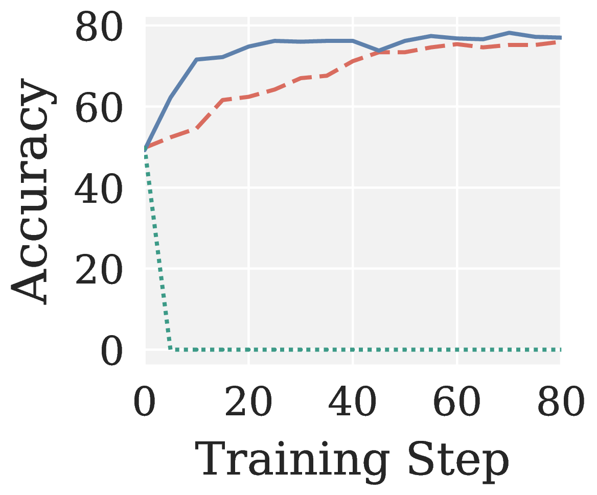
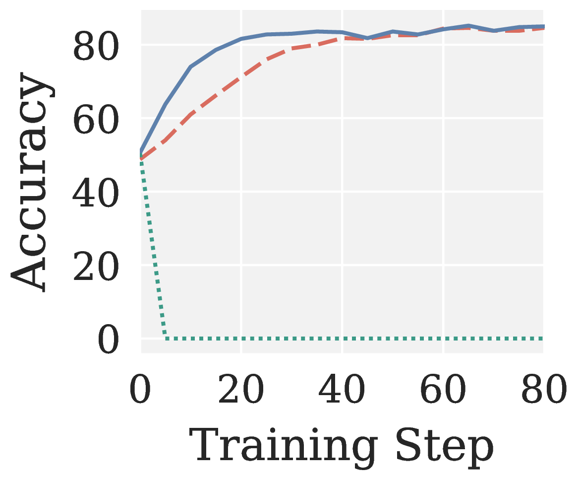
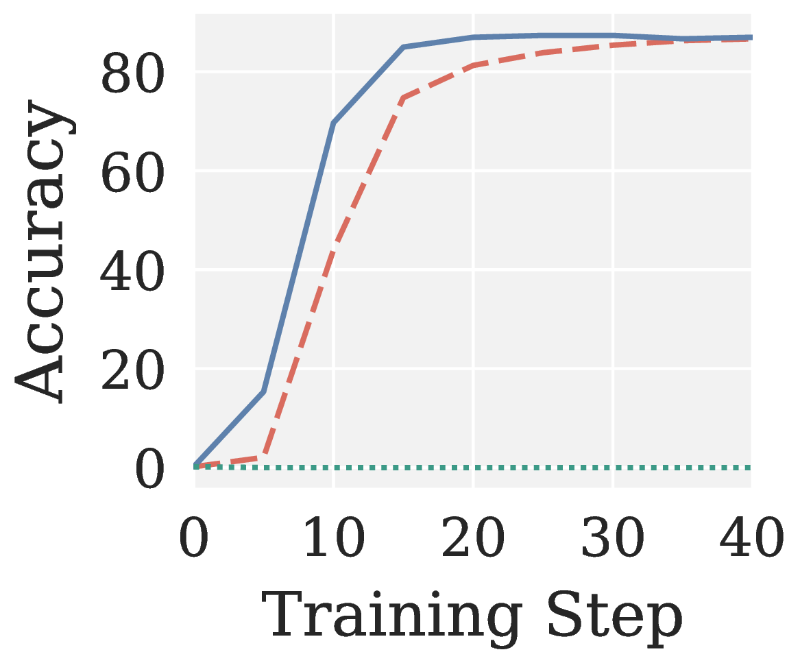
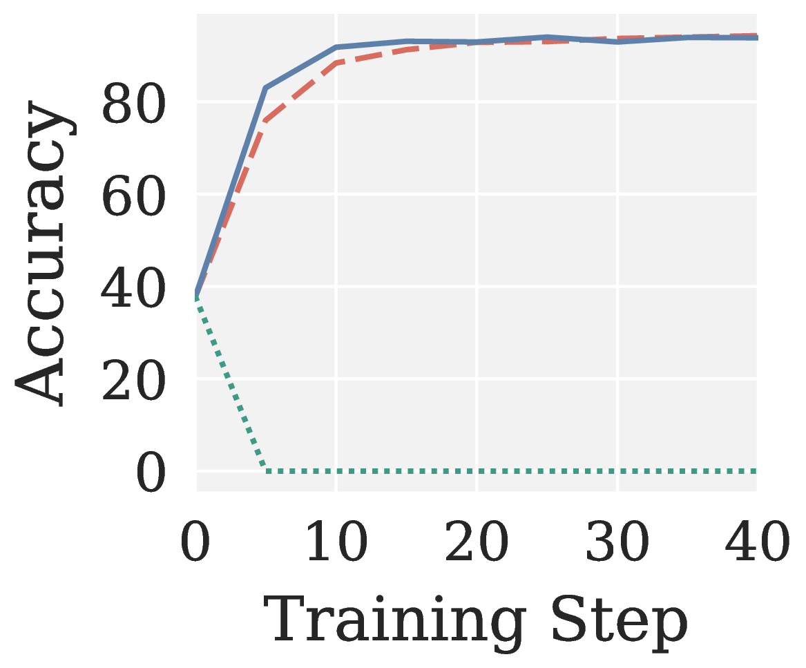
Figure 6. AdamW, Muon, and Pion on RLVR: validation accuracy vs training step across eight settings (two algorithms × two model sizes × two benchmarks).
Reverse ablation: direction of spectral shaping matters. To verify that the gains come specifically from the high-pass direction, we construct Low-pass Muon (LPMuon), which shares Pion’s NS structure and per-step cost but reverses the filtering direction to low-pass (contracting large singular values and amplifying small ones). LPMuon fails to train: its accuracy stays at the initial checkpoint, see Figure 7.
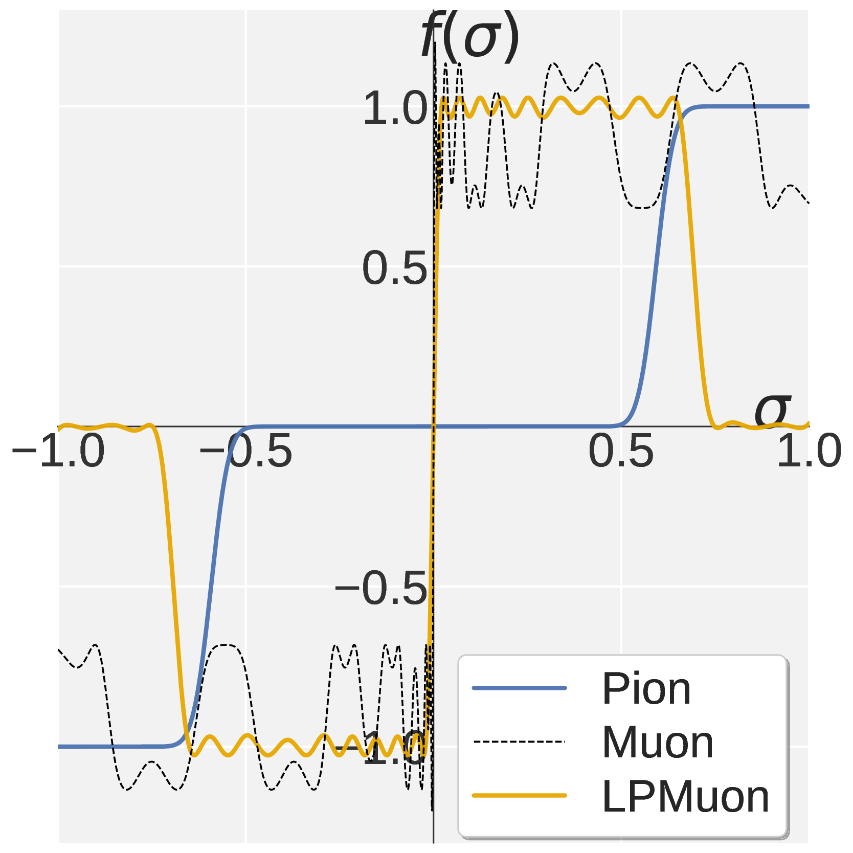
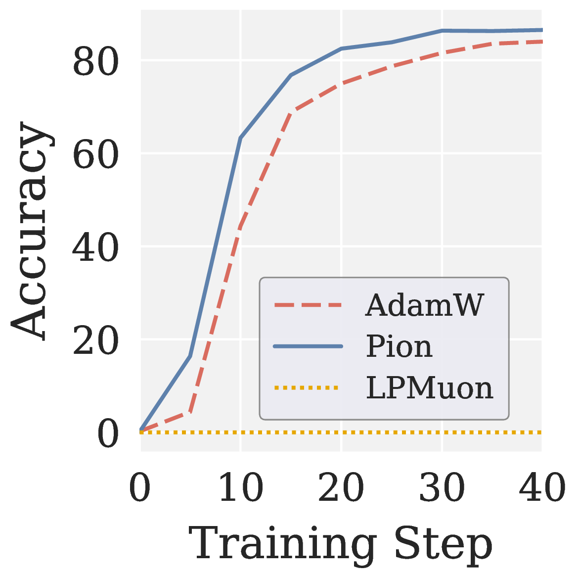
Figure 7. (a) Scalar map \(f(\sigma)\) of LPMuon. (b) GSM8K accuracy of AdamW, Pion, and LPMuon (Qwen3 1.7B, GRPO).
BibTeX
@misc{fan2026rethinkingmuonpretrainingspectral,
      title={Rethinking Muon Beyond Pretraining: Spectral Failures and High-Pass Remedies for VLA and RLVR},
      author={Chongyu Fan and Gaowen Liu and Mingyi Hong and Ramana Rao Kompella and Sijia Liu},
      year={2026},
      eprint={2605.19282},
      archivePrefix={arXiv},
      primaryClass={cs.LG},
      url={https://arxiv.org/abs/2605.19282},
}
TL;DR
- Muon 是一种在 LLM 预训练中被广泛采用的“矩阵感知”优化器。它通过 Newton–Schulz (NS) 迭代将所有奇异值统一放大至 1 附近,从而实现动量矩阵正交化。
- 然而我们发现,这种“一刀切”放大所有奇异值的做法具有局限性,一旦脱离 LLM 预训练设定(如更换模态、损失或学习范式)便不再适用。
- 为此,我们提出 Pion(sPectral hIgh-pass Optimization on momeNtum)。该方法仅需修改 Muon 中 NS 迭代的系数,在保持每步计算开销与 Muon 完全一致的前提下,实现了一种“谱高通”机制,也就是将承载主要信息的头部奇异值锚定在 1 附近,并将噪声主导的尾部奇异值抑制至 0。
试一试:σ 被映射到何处?
背景
Muon
Muon 是一种”矩阵感知“优化器,在 LLM 预训练中应用广泛。记权重矩阵为 \(\boldsymbol{\Theta} \in \mathbb{R}^{m \times n}\),梯度为 \(\mathbf{G}_t\),动量为 \(\mathbf{M}_t = \mu \mathbf{M}_{t-1} + \mathbf{G}_t\)。Muon 在谱范数下执行最速下降:
\[\boldsymbol{\Theta}_t = \boldsymbol{\Theta}_{t-1} - \eta \, \mathrm{msign}(\mathbf{M}_t).\]若 \(\mathbf{M} = \mathbf{U} \boldsymbol{\Sigma} \mathbf{V}^\top\) 为其紧凑 SVD,则
\[\mathrm{msign}(\mathbf{M}) = \mathbf{U}\, \mathrm{sign}(\boldsymbol{\Sigma})\, \mathbf{V}^\top = \mathbf{U} \mathbf{V}^\top.\]所有非零奇异值均被映射至 1 附近,即所谓的均匀谱白化。然而在大模型训练中,每步执行一次 SVD 代价过高,因此 Muon 转而用若干步 NS 迭代近似 \(\mathrm{msign}\)。先将输入归一化为 \(\mathbf{X} \leftarrow \mathbf{X} / (\|\mathbf{X}\|_F + \epsilon)\),再在每一步 NS 中应用一次奇次多项式:
\[\mathbf{X} \leftarrow a\, \mathbf{X} + b\, \mathbf{X}\mathbf{X}^\top \mathbf{X} + c\, \mathbf{X}(\mathbf{X}^\top \mathbf{X})^2,\]系数取 \((a, b, c) = (3.4445,\ -4.7750,\ 2.0315)\)。借助恒等式 \(\mathbf{X}(\mathbf{X}^\top \mathbf{X})^j = \mathbf{U}\, \boldsymbol{\Sigma}^{2j+1}\, \mathbf{V}^\top\),每一步 NS 都保持奇异向量不变,仅通过 \([0, 1]\) 上的一个标量多项式对奇异值进行重塑:
\[f(\sigma;\, a, b, c) \,\triangleq\, a\sigma + b\sigma^3 + c\sigma^5.\]Muon 的 NS 能将任意 \(\sigma \in (0, 1]\) 放大到 1 附近。该函数的图像见 图 1。
Muon 在其他场景下是否仍然适用?
LLM 预训练通常使用 next token prediction loss;更具体地说,任务是分类,模态只有文本,范式是监督学习。当 token 级监督密集且准确时,将所有奇异值放大到 1 是较为合理的默认选择。但 LLM 预训练只是深度学习的一部分,Muon 在不同模态、不同损失、不同学习范式下的表现,仍是值得探索的问题:
动机
我们考虑了两个 setting:VLA 与 RLVR。VLA 同时改变了模态与损失(引入视觉与动作模态,并将分类损失替换为回归损失);RLVR 则单独改变学习范式(将监督学习替换为强化学习)。通过对梯度秩和信噪比的分析,我们发现 Muon 在动作模态和强化学习场景下均不适用。
更换模态与损失:VLA
VLA 模型由三部分构成:vision encoder、language backbone 与 action head。vision 与 language 模块的输入是文本指令与图像;action head 则对应一种全新的模态,其输出是机器人的动作。相应地,action head 通常采用的是非分类损失:要么是 \(\ell_1\) regression,要么是 flow matching。
我们用有效秩(effective rank, erank)来刻画各模块梯度 \(\mathbf{G} \in \mathbb{R}^{m \times n}\) 的谱结构:
\[\mathrm{erank}(\mathbf{G}) \,\triangleq\, \exp\!\Big( H(\mathbf{p}) \Big), \quad H(\mathbf{p}) = -\sum_{i=1}^n p_i \log p_i, \quad p_i = \frac{\sigma_i(\mathbf{G})}{\sum_j \sigma_j(\mathbf{G})}.\]erank 越大,说明梯度的能量分散在很多奇异方向上;越小,说明能量集中在少数几个主方向上。
图 2. Muon 在 VLA 训练(VLA Adapter + LIBERO Object)中的局限性。(a) 全模态使用 AdamW 训练时,各模态梯度的有效秩 (erank)。(b)(c) 4.5k 步时的测试成功率与总训练时长(其中 vision 和 language 使用 AdamW,仅切换 action 的优化器)。
从 图 2(a) 可以看出,各模态梯度的 erank 在整个训练过程中非常稳定:vision 最高、language 居中,而action 梯度的 erank 始终最低。这主要是因为 vision 与 text 输入通常包含更丰富的信息,而 action 仅需 7 个自由度即可表达;此外,action 模态采用的是 regression loss 进行训练,其输出空间远小于 language 与 vision 的离散 token 空间,这使其梯度展现出极强的低秩特性。在这种低秩的 action 梯度上直接施加 Muon 的均匀白化,等同于将微弱的噪声尾部抬升至与少数主方向相同的量级,导致最终的参数更新几乎完全被谱底噪声主导。如 图 2(b) 所示,Muon 在 action 模块上的成功率甚至不及 AdamW。一个直观的解决方案是 Low-Rank Muon (LRMuon),即在 NS 迭代之前,先通过 SVD 或 Gaussian sketching 将动量矩阵投影到 top-\(k\) 子空间。这种方法虽能恢复成功率,但 图 2(c) 表明,引入显式低秩投影会带来巨大的计算负担,使整个训练开销激增约一个数量级。
局限 1(modality + loss)。 标准 Muon 无法自适应新模态、新损失所带来的谱秩异质性;显式低秩投影虽能恢复成功率,但代价是失去可扩展性。
更换学习范式:RLVR
RLVR 保持 LLM 与文本模态不变,所改变的仅是学习范式:将 token 级监督损失(如 SFT)替换为轨迹级针对可验证奖励的策略梯度(如 GRPO)。为了将两种学习范式置于同一坐标下比较,我们考察每一步梯度的信噪比:
\[\mathrm{SNR}(\mathbf{G}) \,\triangleq\, \frac{\|\mathbb{E}[\mathbf{G}]\|_F^2}{\mathbb{E}\big[\,\|\mathbf{G} - \mathbb{E}[\mathbf{G}]\|_F^2\,\big]}.\]图 3(a) 中的 SNR 鸿沟有两个结构性来源。一是监督粒度变粗:SFT 使用 token 级教师信号,而 GRPO 使用轨迹级奖励,每个 token 实际获得的学习信号要稀疏得多。二是稳定化机制:importance sampling、clipping、advantage normalization 均会重新加权或抹除部分 per-token 梯度,进一步放大方差。如 图 3(b) 所示,Muon 直接对这种低 SNR 梯度做白化,相当于将噪声方向抬升至与信息方向同等量级,最终策略在数步之内便崩溃。
图 3. RLVR SNR(Qwen3 1.7B,MATH)。(a) 整段训练中 GRPO 的梯度 SNR 始终明显低于 SFT。(b) 在 GRPO 下,AdamW 稳步提升,而 Muon 在数步之内便崩溃至接近零的准确率。
局限 2(learning paradigm)。 Muon 的均匀白化会放大低 SNR 的 RLVR 梯度中的噪声方向,因而不适合对噪声敏感的后训练。
方法
局限 1 与局限 2 的来源不同:前者源于不同 modality / loss 的低 erank,后者源于不同 learning paradigm 的低 SNR;但二者在频谱上呈现出相同的形态。在 \(\mathbf{M}_t\) 的 SVD 中,前若干个奇异值承载着高信息量的下降方向,其余大量小奇异值则被噪声主导(在 erank 较低时表现为谱底,在 SNR 较低时表现为随机估计噪声)。Muon 的 \(\mathrm{msign}\) 将尾部抬升至与头部同等量级,因此在上述两种情形下都会扰乱更新。自然的对策即为谱高通:将头部锚定在 1 附近,将尾部抑制到 0。
高通 NS
由于 NS 每一步都通过 \(f(\sigma; a, b, c) = a\sigma + b\sigma^3 + c\sigma^5\) 重塑 \(\sigma\),因此 NS 的设计归结为对 \(f\) 的设计。仅依靠单一的五次多项式,难以实现我们所需的高通;为此,Pion 将默认的 \(k = 5\) 步 NS 拆分为两段,分别使用不同的系数:
- 第一段称为 Promotion(提升),多项式 \(f_{\mathrm{p}}\) 运行 \(k_{\mathrm{p}}\) 步:放大头部奇异值到 1 附近,同时保留它们之间的相对大小;
- 第二段称为 Suppression(抑制),多项式 \(f_{\mathrm{s}}\) 运行 \(k_{\mathrm{s}} = k - k_{\mathrm{p}}\) 步:将已经接近 1 的大奇异值锚定在 1,将仍偏小的奇异值进一步压制至 0。
我们对 \(f_{\mathrm{p}}\) 给出三条要求:(P1) \(\sigma = 1\) 是不动点,\(f_{\mathrm{p}}(1) = 1\);(P2) 一阶平稳,\(f_{\mathrm{p}}'(1) = 0\);(P3) 边界凹性,\(f_{\mathrm{p}}''(1) \leq 0\),与 (P2) 共同保证 \(\sigma = 1\) 为局部极大点,迭代不会在边界附近越过 1 而发散。(P1) 与 (P2) 将可行解约束为单参数族,进一步结合 (P3) 与 \([0, 1]\) 上的单调性,可行参数收缩为 \(a_{\mathrm{p}} \in [0, 1.875]\)。\(f_{\mathrm{p}}'(0) = a_{\mathrm{p}}\) 控制每一步对小奇异值的提升强度,因此我们直接取其最大可行斜率,从而唯一确定多项式:
\[f_{\mathrm{p}}(\sigma) = 1.875\, \sigma \,-\, 1.25\, \sigma^3 \,+\, 0.375\, \sigma^5.\]由于其导数恰为完全平方 \(f_{\mathrm{p}}'(\sigma) = 1.875\, (1 - \sigma^2)^2 \geq 0\),单调性自然成立。
Suppression 同样要求 \(f_{\mathrm{s}}(1) = 1\)、\(f_{\mathrm{s}}'(1) = 0\),并附加一条谱过滤条件:\(f_{\mathrm{s}}'(0) = 0\)。在消除原点附近的线性项之后,小奇异值仅能被高阶项逐步缩小到 0。其唯一解为:
\[f_{\mathrm{s}}(\sigma) = 2.5\, \sigma^3 \,-\, 1.5\, \sigma^5.\]将 \(k_{\mathrm{p}}\) 步 Promotion 与 \(k_{\mathrm{s}}\) 步 Suppression 串联,即可得到 Pion 的高通 NS。固定 \(k = 5\) 使其每步开销与 Muon 完全一致。图 1 给出了 Muon NS、Promotion、Suppression 与 Pion 高通 NS 的函数图像对比。
图 1. \(\sigma \in [0, 1]\) 上 \(f(\sigma)\) 的可视化。Muon (a) 将每一个奇异值都放大到 1。Pion 将 Promotion (b) 与 Suppression (c) 组合,得到 (d) 中的高通形态。
Per-head 模式(用于 RLVR)
目前为止,高通 NS 都将每一层的动量 \(\mathbf{M}_t \in \mathbb{R}^{m \times n}\) 作为单一整块处理,与 Muon 完全一致;我们称之为 default mode。但我们发现,这种方式并不适用于 RLVR。RLVR 起点是已经 pretrained(或 SFT 过的)LLM,其 attention 层各 head 之间在 \(\|\mathbf{W}_Q^h\|_F\)、\(\|\mathbf{W}_K^h\|_F\)、\(\|\mathbf{W}_V^h\|_F\)、\(\|\mathbf{W}_O^h\|_F\) 上存在显著差异。这种差异同时决定了 forward 的输出与 backward 的梯度,因此不同 head 本应接收不同尺度的更新。
为此,Pion 在 default mode 之外提供一种 per-head mode:先沿 head 维度将 attention 投影 reshape 为若干 per-head 子矩阵,再分别在每一个子矩阵上独立运行整套两段式高通 NS。形式上,设 \(H\) 为 attention head 数、\(d_k\) 为单 head 维度,每个 attention 投影(Q / K / V / O 任一)都有一个沿 head 轴的标准 reshape:
\[\mathbf{M}_t \;\xrightarrow{\;\mathrm{Reshape}\;}\; \{\mathbf{M}_t^h\}_{h=1}^{H}, \qquad \mathbf{M}_t^h \in \mathbb{R}^{d \times d_k}.\]Per-head mode 在每个 \(\mathbf{M}_t^h\) 上独立执行两段式高通 NS:先做 per-head 的 Frobenius 预归一化 \(\mathbf{X}^h \leftarrow \mathbf{M}_t^h / (\|\mathbf{M}_t^h\|_F + \epsilon)\),再依次执行 \(k_{\mathrm{p}}\) 步 Promotion 与 \(k_{\mathrm{s}}\) 步 Suppression,最后再将 \(\{\mathbf{X}^h\}_{h=1}^H\) reshape 回完整的 \(\mathbf{X} \in \mathbb{R}^{m \times n}\)。由于 \(\mathbf{X}^h (\mathbf{X}^h)^\top \mathbf{X}^h\) 在 GPU 上本就沿 \(h\) 维做了 batch,per-head mode 相对 default mode 的唯一额外开销即为 reshape 本身。
图 4(a) 在 Qwen3 1.7B 上具体展示了 default mode 的问题:RLVR 起点权重的跨 head 方差 \(\mathrm{Var}_h(\|\mathbf{W}_{0,Q}^h\|_F)\) 在全部 28 层都不可忽略(上方),但在 default mode 的 Pion 下,更新量的跨 head 方差 \(\mathrm{Var}_h(\|\mathbf{W}_{*,Q}^h - \mathbf{W}_{0,Q}^h\|_F)\) 几乎为零(下方)。也就是说,default mode 会拉平各 head 的更新尺度,并把不同 head 的子方向混合在一起,使得各 head 都得到几乎相同的更新,完全无法体现 head 之间的差异性。相比之下,per-head mode 则恢复了与层相关、随 head 变化的更新结构。
图 4. Per-head 高通 NS 在 RLVR 上的效果(Qwen3 1.7B,GRPO + MATH 难度 3 至 5)。(a) Q 投影的跨 head 方差:RLVR 之前 \(\mathrm{Var}_h(\|\mathbf{W}_{0,Q}^h\|_F)\)(上)与 RLVR 更新量 \(\mathrm{Var}_h(\|\mathbf{W}_{*,Q}^h - \mathbf{W}_{0,Q}^h\|_F)\) 在 default 与 per-head Pion 下的对比(下)。(b) AdamW、Muon(default vs per-head)、Pion(default vs per-head)的 MATH500 准确率。
至此,Pion 的 per-head 高通 NS 包含两个设计:谱高通与 per-head reshape。一个自然的问题是:两者谁更关键?我们发现两者互补但并不对称。谱高通是 Pion 提升的主要驱动:在 图 4(b) 中,即便给 Muon 的 NS 也加上同样的 reshape,得到的 per-head Muon 依然完全崩溃,因为它逐 head 注入的噪声尾部,与它在整块矩阵上注入的噪声同样致命。Per-head reshape 则是辅助机制,用于保留 pretrained(或 SFT 过的)LLM 中 attention 层各 head 的差异性。
伪代码
算法 1 是 Muon 标准的 NS 迭代;算法 2 是 Pion 高通 NS 的默认模式,算法 3 是 per-head 模式。 Pion 与 Muon 的差异 per-head 模式独有
- \(\mathbf{M}_0 \leftarrow \mathbf{0}\)
- for \(t = 1, 2, \dots\) do
- \(\mathbf{G}_t \leftarrow \nabla_{\boldsymbol{\Theta}} \mathcal{L}_t(\boldsymbol{\Theta}_{t-1})\)
- \(\mathbf{M}_t \leftarrow \mu\, \mathbf{M}_{t-1} + \mathbf{G}_t\)
- \(\mathbf{X} \leftarrow \mathbf{M}_t / (\lVert \mathbf{M}_t \rVert_F + \epsilon)\)谱预归一化
- for \(i = 1, \dots, k\) do\((a, b, c) = (3.4445, -4.7750, 2.0315)\)
- \(\mathbf{X} \leftarrow a\mathbf{X} + b\mathbf{X}\mathbf{X}^\top\mathbf{X} + c\mathbf{X}(\mathbf{X}^\top\mathbf{X})^2\)
- end for
- \(\boldsymbol{\Theta}_t \leftarrow \boldsymbol{\Theta}_{t-1} - \eta\, \mathbf{X}\)
- end for
- return \(\boldsymbol{\Theta}_t\)
- \(k_{\mathrm{s}} \leftarrow 5 - k_{\mathrm{p}}\)把 \(k = 5\) 拆成 \(k_{\mathrm{p}} + k_{\mathrm{s}}\)
- \(\mathbf{M}_0 \leftarrow \mathbf{0}\)
- for \(t = 1, 2, \dots\) do
- \(\mathbf{G}_t \leftarrow \nabla_{\boldsymbol{\Theta}} \mathcal{L}_t(\boldsymbol{\Theta}_{t-1})\)
- \(\mathbf{M}_t \leftarrow \mu\, \mathbf{M}_{t-1} + \mathbf{G}_t\)
- \(\mathbf{X} \leftarrow \mathbf{M}_t / (\lVert \mathbf{M}_t \rVert_F + \epsilon)\)谱预归一化
- for \(i = 1, \dots, k_{\mathrm{p}}\) do第一阶段 Promotion,\((a_{\mathrm{p}}, b_{\mathrm{p}}, c_{\mathrm{p}}) = (1.875, -1.25, 0.375)\)
- \(\mathbf{X} \leftarrow a_{\mathrm{p}}\mathbf{X} + b_{\mathrm{p}}\mathbf{X}\mathbf{X}^\top\mathbf{X} + c_{\mathrm{p}}\mathbf{X}(\mathbf{X}^\top\mathbf{X})^2\)
- end for
- for \(j = 1, \dots, k_{\mathrm{s}}\) do第二阶段 Suppression,\((a_{\mathrm{s}}, b_{\mathrm{s}}, c_{\mathrm{s}}) = (0, 2.5, -1.5)\)
- \(\mathbf{X} \leftarrow a_{\mathrm{s}}\mathbf{X} + b_{\mathrm{s}}\mathbf{X}\mathbf{X}^\top\mathbf{X} + c_{\mathrm{s}}\mathbf{X}(\mathbf{X}^\top\mathbf{X})^2\)
- end for
- \(\boldsymbol{\Theta}_t \leftarrow \boldsymbol{\Theta}_{t-1} - \eta\, \mathbf{X}\)
- end for
- return \(\boldsymbol{\Theta}_t\)
- \(k_{\mathrm{s}} \leftarrow 5 - k_{\mathrm{p}}\)把 \(k = 5\) 拆成 \(k_{\mathrm{p}} + k_{\mathrm{s}}\)
- \(\mathbf{M}_0 \leftarrow \mathbf{0}\)
- for \(t = 1, 2, \dots\) do
- \(\mathbf{G}_t \leftarrow \nabla_{\boldsymbol{\Theta}} \mathcal{L}_t(\boldsymbol{\Theta}_{t-1})\)
- \(\mathbf{M}_t \leftarrow \mu\, \mathbf{M}_{t-1} + \mathbf{G}_t\)
- \(\{\mathbf{M}_t^h\}_{h=1}^{H} \leftarrow \mathrm{Reshape}(\mathbf{M}_t)\)沿 head 维度切分
- \(\mathbf{X}^h \leftarrow \mathbf{M}_t^h / (\lVert \mathbf{M}_t^h \rVert_F + \epsilon),\ \forall\, h\)per-head 预归一化
- for \(i = 1, \dots, k_{\mathrm{p}}\) do第一阶段 Promotion,沿 \(H\) batch
- \(\mathbf{X}^h \leftarrow a_{\mathrm{p}}\mathbf{X}^h + b_{\mathrm{p}}\mathbf{X}^h(\mathbf{X}^h)^\top\mathbf{X}^h + c_{\mathrm{p}}\mathbf{X}^h\bigl((\mathbf{X}^h)^\top\mathbf{X}^h\bigr)^2\)
- end for
- for \(j = 1, \dots, k_{\mathrm{s}}\) do第二阶段 Suppression,沿 \(H\) batch
- \(\mathbf{X}^h \leftarrow a_{\mathrm{s}}\mathbf{X}^h + b_{\mathrm{s}}\mathbf{X}^h(\mathbf{X}^h)^\top\mathbf{X}^h + c_{\mathrm{s}}\mathbf{X}^h\bigl((\mathbf{X}^h)^\top\mathbf{X}^h\bigr)^2\)
- end for
- \(\mathbf{X} \leftarrow \mathrm{Reshape}^{-1}(\{\mathbf{X}^h\}_{h=1}^{H})\)合并 per-head 矩阵
- \(\boldsymbol{\Theta}_t \leftarrow \boldsymbol{\Theta}_{t-1} - \eta\, \mathbf{X}\)
- end for
- return \(\boldsymbol{\Theta}_t\)
实验
我们在两个 setting 验证 Pion:
- VLA 训练:两种结构,基于 \(\ell_1\)-regression 的 VLA Adapter 与基于 flow-matching 的 VLANeXt,以 LIBERO 和 LIBERO Plus 作为 benchmark;
- RLVR 后训练:算法选用 GRPO 和 GMPO;模型选用 Qwen3 1.7B 和 Qwen3 4B;benchmark 为 MATH 和 GSM8K。
VLA
VLA Adapter on LIBERO。 我们首先在 VLA Adapter 上对 AdamW、Muon、Pion 进行比较:在 LIBERO 的四个子集(Object、Spatial、Goal、Long)上,每个子集采用固定训练预算(Object 1,500 步,其余 15,000 步),并在 Object 上额外给出更精细的训练曲线。
图 5. AdamW、Muon、Pion 用于 VLA Adapter on LIBERO。(a) LIBERO Object、Spatial、Goal、Long 四个子集上的成功率,每个子集采用固定的训练预算(Object 1,500 步,其余 15,000 步)。(b) LIBERO Object 上的成功率 vs 训练步数。
图 5(a) 表明,Pion 在每个子集上都全面优于 Muon 和 AdamW。图 5(b) 进一步给出 LIBERO Object 上的训练曲线:Pion 在 500 步即达到 95.4% 成功率,并在 1,500 步时饱和至 100%;AdamW 则需要明显更多的步数才能逼近。这说明谱高通大幅降低了到达高成功率所需的训练成本。
在 VLANeXt(flow matching)上,Pion 不仅在 LIBERO 上取得最佳成功率,在更具挑战性的 LIBERO Plus 上也能继续保持优势,尤其是 language(\(+9\) 分)、noise(\(+6\) 分)、robot(\(+6\) 分)等几项扰动;详见 表 1。这恰好印证了我们之前的判断:均匀白化会过度放大那些无法泛化的噪声方向。
| 优化器 | LIBERO | LIBERO Plus | Background | Camera | Language | Layout | Light | Noise | Robot |
|---|---|---|---|---|---|---|---|---|---|
| AdamW | 79.45 | 64.57 | 68.97 | 70.38 | 54.50 | 61.80 | 76.35 | 66.37 | 47.04 |
| Muon | 93.65 | 72.34 | 82.72 | 68.00 | 77.53 | 76.21 | 86.17 | 69.98 | 57.36 |
| Pion (Ours) | 96.35 | 75.93 | 84.53 | 70.88 | 86.93 | 76.71 | 90.67 | 76.09 | 63.18 |
表 1. AdamW、Muon、Pion 用于 VLANeXt on LIBERO 与 LIBERO Plus。每列最优用粗体。
为了把 LIBERO Plus 上的差距更直观地展示出来,我们在同一个 LIBERO Plus episode 上,让三种优化器各自训练得到的 VLANeXt 策略各 rollout 一次。AdamW 与 Muon 在抓取或放置阶段失败,而 Pion 顺利完成任务。
视频 1. LIBERO Plus 同一个 episode(ep1373)在 AdamW、Muon、Pion 三种优化器训练得到的 VLANeXt 策略下的 rollout 轨迹。
RLVR
在全部 8 个 RLVR setting 上(GRPO/GMPO × Qwen3 1.7B/4B × MATH/GSM8K,见 图 6),Muon 无一例外地崩溃至接近零的准确率;Pion 不仅恢复出有意义的训练信号,收敛速度也快于 AdamW。
图 6. RLVR 上 AdamW、Muon、Pion 的验证准确率 vs 训练步:8 个 setting(两种算法 × 两种模型规模 × 两个 benchmark)。
反向消融:方向才是关键。 为确认增益的确来自”高通”这一方向,我们构造了 Low-pass Muon (LPMuon):它与 Pion 共享 NS 结构与每步开销,但将滤波方向反转为低通。结果 LPMuon 完全无法训练,准确率始终停留在初始 checkpoint 水平,见 图 7。
图 7. (a) LPMuon 的标量映射 \(f(\sigma)\)。(b) AdamW、Pion、LPMuon 的 GSM8K 准确率(Qwen3 1.7B,GRPO)。
BibTeX
@misc{fan2026rethinkingmuonpretrainingspectral,
      title={Rethinking Muon Beyond Pretraining: Spectral Failures and High-Pass Remedies for VLA and RLVR},
      author={Chongyu Fan and Gaowen Liu and Mingyi Hong and Ramana Rao Kompella and Sijia Liu},
      year={2026},
      eprint={2605.19282},
      archivePrefix={arXiv},
      primaryClass={cs.LG},
      url={https://arxiv.org/abs/2605.19282},
}